Metabarcoding workflow for 18S amplicon sequencing

The 18S region contains many different regions to pick from for metabarcoding. The Ecosystem team at GMGI has optimized the 18S SSU set (18S-SSU-F04, 18S-SSU-R22) and the 18S-v8v9 set (18S-1422F, 18S-1797R). Due to better species coverage, the GMGI Ecosystem Team has switched over to using the v8v9 region for 18S.

Citations:
- 18S-SSU-F04, 18S-SSU-R22 [Blaxter et al. 1998/Fonseca et al. 2010]
- 18S-1422F, 18S-1797R [Bradley et al. 2016]

Analysis workflow:
1. Assess quality of fastq files using FASTQC and MultiQC
2. Identify sequencing outliers and sub-sample if needed
3. Run nf-core/ampliseq to remove adapters, predict ASVs, assign taxonomy, and generate counts tables

Project set-up

Typical project folder structure (once analysis is run) for Fisheries team. Create scripts, results (for ampliseq output), fastqc, and metadata. E.g., mkdir results.

fastqc  metadata  multiqc_raw_data  multiqc_raw.html  raw_data  results  scripts

Create/edit a slurm script: nano name.sh
View a file without editing: less name.sh
Start an interactive node: srun --pty bash

Confirm conda environment is available

The conda environment is started within each slurm script, but to activate conda environment outside of the slurm script to update packages or check what is installed:

# Activate conda
source /projects/gmgi/miniconda3/bin/activate

# Activate fisheries eDNA conda environment 
conda activate fisheries_eDNA

# List all available environments 
conda env list 

# List all packages installed in fisheries_eDNA
conda list 

# Update a package
conda update [package name]

# Update nextflow ampliseq workflow 
nextflow pull nf-core/ampliseq

Assess quality of raw data

Background information on FASTQC. This should take ~10 seconds per file for a typical full MiSeq run. If <2 seconds, then check output/error files.

Create slurm script: nano 01-fastqc.sh. Copy below script into file and save (Ctrl+X; Y; Enter).

#!/bin/bash
#SBATCH --error=output/fastqc_output/"%x_error.%j" #if your job fails, the error report will be put in this file
#SBATCH --output=output/fastqc_output/"%x_output.%j" #once your job is completed, any final job report comments will be put in this file
#SBATCH --partition=short
#SBATCH --nodes=1
#SBATCH --time=20:00:00
#SBATCH --job-name=fastqc
#SBATCH --mem=3GB
#SBATCH --ntasks=1
#SBATCH --cpus-per-task=2

### USER TO-DO ### 
## 1. Set paths for your project

# Activate conda environment
source /projects/gmgi/miniconda3/bin/activate fisheries_eDNA

## SET PATHS (USER EDITS)
raw_path="/projects/gmgi/example/18S/raw_data"
out_dir="/projects/gmgi/example/18S/fastqc"

## CREATE SAMPLE LIST FOR SLURM ARRAY
### 1. Create list of all .gz files in raw data path
ls -d ${raw_path}/*.gz > ${raw_path}/rawdata

### 2. Create a list of filenames based on that list created in step 1
mapfile -t FILENAMES < ${raw_path}/rawdata

### 3. Create variable i that will assign each row of FILENAMES to a task ID
i=${FILENAMES[$SLURM_ARRAY_TASK_ID]}

## RUN FASTQC PROGRAM 
fastqc ${i} --outdir ${out_dir}

To run:
- Start slurm array (e.g., with 138 files) = sbatch --array=0-137 01-fastqc.sh. Note that this starts with file 0.

Count the number of files by navigating to raw data folder and using ls *.gz | wc. The first column is the number of rows in the generated list (files).

Notes:

• This is going to output many error and output files. After job completes, navigate to cd scripts/output/fastqc_output and use cat *output.* > ../fastqc_output.txt to create one file with all the output and cat *error.* > ../fastqc_error.txt to create one file with all of the error message outputs.
• Within the out_dir output folder, use ls *html | wc to count the number of html output files (1st/2nd column values). This should be equal to the --array range used and the number of raw data files. If not, the script missed some input files so address this before moving on.

Visualize quality of raw data

Background information on MULTIQC.

Run the following code in an interactive node. This program will be quick for eDNA data (typically <2 minutes).

# Use srun to claim a node
srun --pty bash 

# Activate conda environment
source /projects/gmgi/miniconda3/bin/activate fisheries_eDNA

## SET PATHS 
## fastqc_output = output from 00-fastqc.sh; fastqc program
fastqc_output="" 
multiqc_dir="" 

## RUN MULTIQC 
### Navigate to your project
multiqc --interactive ${fastqc_output} -o ${multiqc_dir} --filename multiqc_raw.html

Path examples:
- fastqc_output="/projects/gmgi/example/fastqc"
- multiqc_dir="/projects/gmgi/example" (goes in general folder)

Identify sequencing outliers and sub-sample if needed

This step can be done two ways: 1) download read counts from Illumina basespace run information or 2) Download read counts from the multiqc report. Either way, you need an excel file with the sample ID and total read count.

Read counts can be downloaded from the General Statistics section on Multiqc by selecting Export as CSV > Data > Format (csv) > Download Plot Data. Save this file in the project repository.

We use a median absolute deviation (MAD) approach that works by first finding the median of the data, then measuring how far each value deviates from that median and using the median of those deviations as the typical spread. Values whose deviation is much larger than this typical spread are flagged as outliers.

Visit this page for the R script or download here.

Download seqtk program

This program has already been installed on NU with the below code:

# move to gmgi/packages folder 
cd /projects/gmgi/packages/

# download seqtk program from their github page; move into that folder; and enable (`make`) the program
# ; indicates a pipe much like %>% in R
git clone https://github.com/lh3/seqtk.git;
cd seqtk; make

Path to the program: /projects/gmgi/packages/seqtk/seqtk

Running seqtk with a single (or handful) of samples

Calculate the median number of reads prior to this code. This example will use 70,377.

# start an interactive session on 1 node
srun --pty bash 

# cd to your raw data folder
# make a new folder called outliers (`mkdir` = make directory)
mkdir outliers

# define a path to reference later using ${seqtk}
seqtk="/projects/gmgi/packages/seqtk/seqtk"

# reference the program path above using ${} and subsample the original fastq file 
# to 70,377 reads using a set seed of -s100 following by gzipping that file using a pipe |
# that is similar to %>% in R. I have two commands then: 1) sub-sample 2) gzip 
# > indicates a new output file 

${seqtk} sample -s100 INS2-FS-0011_S284_L001_R1_001.fastq.gz 70377 | gzip > INS2-FS-0011_S284_L001_R1_001_subset.fastq.gz
${seqtk} sample -s100 INS2-FS-0011_S284_L001_R2_001.fastq.gz 70377 | gzip > INS2-FS-0011_S284_L001_R2_001_subset.fastq.gz

# move original files into the outliers folders so they are out of the way of our analysis 
mv INS2-FS-0011_S284_L001_R1_001.fastq.gz outliers/
mv INS2-FS-0011_S284_L001_R2_001.fastq.gz outliers/

Running seqtk with a list of files

Create a samplesheet using 03a-metadata.R below as an example. If you have a csv with 'sampleID', 'forwardReads', and 'reverseReads' columns then turn that csv into a text file with:

tail -n +2 outlier_list_for_subsampling.csv | cut -d',' -f2,3 | tr ',' '\n' > outlier_paths.txt

The input to the below .sh is a txt file with a single column with no header that lists the full path of each fastq file to subset.

02-outlier.sh

#!/bin/bash
#SBATCH --error=output/"%x_error.%j" #if your job fails, the error report will be put in this file
#SBATCH --output=output/"%x_output.%j" #once your job is completed, any final job report comments will be put in this file
#SBATCH --partition=short
#SBATCH --nodes=1
#SBATCH --time=4:00:00
#SBATCH --job-name=02-outlier
#SBATCH --mem=1GB
#SBATCH --ntasks=1
#SBATCH --cpus-per-task=1

### Running seqtk for a list of files

# path to seqtk
seqtk="/projects/gmgi/packages/seqtk/seqtk"

# input list
input_list="/projects/gmgi/example/18S/outlier_paths.txt"

# directory for subset files 
output_directory="/projects/gmgi/example/18S/raw_data"

# directory to archive files
archive_directory="/projects/gmgi/oceanX/example/18S/raw_data/outliers"

# number of reads
nreads=70377
seed=100

# Run seqtk on the input_list files
while read -r fq; do
    [[ -z "$fq" ]] && continue

    base=$(basename "$fq" .fastq.gz)
    out="${output_directory}/${base}_subset.fastq.gz"

    echo "Subsampling: $fq -> $out"
    "${seqtk}" sample -s"${seed}" "$fq" "${nreads}" | gzip > "$out"

done < "$input_list"


# Move input_list files to the archive folder
mkdir -p "$archive_directory"

while read -r fq; do
    [[ -z "$fq" ]] && continue

    echo "Archiving: $fq -> $archive_directory"
    mv "$fq" "$archive_directory/"

done < "$input_list"

Downloading and updating reference databases

Download and/or update pr2 database

[https://pr2-database.org/]

nf-core/ampliseq will download pr2 on its own, but see below website to confirm that the most recent version was indeed used in your workflow. After ampliseq, view the contents of this file:

/results/dada2/ref_taxonomy.pr2.txt

--dada_ref_taxonomy: pr2

Title: PR2 - Protist Reference Ribosomal Database - Version 5.1.0

Citation: Guillou L, Bachar D, Audic S, Bass D, Berney C, Bittner L, Boutte C, Burgaud G, de Vargas C, Decelle J, Del Campo J, Dolan JR, Dunthorn M, Edvardsen B, Holzmann M, Kooistra WH, Lara E, Le Bescot N, Logares R, Mahé F, Massana R, Montresor M, Morard R, Not F, Pawlowski J, Probert I, Sauvadet AL, Siano R, Stoeck T, Vaulot D, Zimmermann P, Christen R. The Protist Ribosomal Reference database (PR2): a catalog of unicellular eukaryote small sub-unit rRNA sequences with curated taxonomy. Nucleic Acids Res. 2013 Jan;41(Database issue):D597-604. doi: 10.1093/nar/gks1160. Epub 2012 Nov 27. PMID: 23193267; PMCID: PMC3531120.

All entries: [title:PR2 - Protist Reference Ribosomal Database - Version 5.1.0, file:[https://github.com/pr2database/pr2database/releases/download/v5.1.0.0/pr2_version_5.1.0_SSU_dada2.fasta.gz, https://github.com/pr2database/pr2database/releases/download/v5.1.0.0/pr2_version_5.1.0_SSU_UTAX.fasta.gz], citation:Guillou L, Bachar D, Audic S, Bass D, Berney C, Bittner L, Boutte C, Burgaud G, de Vargas C, Decelle J, Del Campo J, Dolan JR, Dunthorn M, Edvardsen B, Holzmann M, Kooistra WH, Lara E, Le Bescot N, Logares R, Mahé F, Massana R, Montresor M, Morard R, Not F, Pawlowski J, Probert I, Sauvadet AL, Siano R, Stoeck T, Vaulot D, Zimmermann P, Christen R. The Protist Ribosomal Reference database (PR2): a catalog of unicellular eukaryote small sub-unit rRNA sequences with curated taxonomy. Nucleic Acids Res. 2013 Jan;41(Database issue):D597-604. doi: 10.1093/nar/gks1160. Epub 2012 Nov 27. PMID: 23193267; PMCID: PMC3531120., fmtscript:taxref_reformat_pr2.sh, dbversion:PR2 v5.1.0 (https://github.com/pr2database/pr2database/releases/tag/v5.1.0.0), taxlevels:Domain,Supergroup,Division,Subdivision,Class,Order,Family,Genus,Species]

Step 4: nf-core/ampliseq

Nf-core: A community effort to collect a curated set of analysis pipelines built using Nextflow.
Nextflow: scalable and reproducible scientific workflows using software containers, used to build wrapper programs like the one we use here.

[https://nf-co.re/ampliseq/2.11.0]: nfcore/ampliseq is a bioinformatics analysis pipeline used for amplicon sequencing, supporting denoising of any amplicon and supports a variety of taxonomic databases for taxonomic assignment including 16S, ITS, CO1 and 18S.

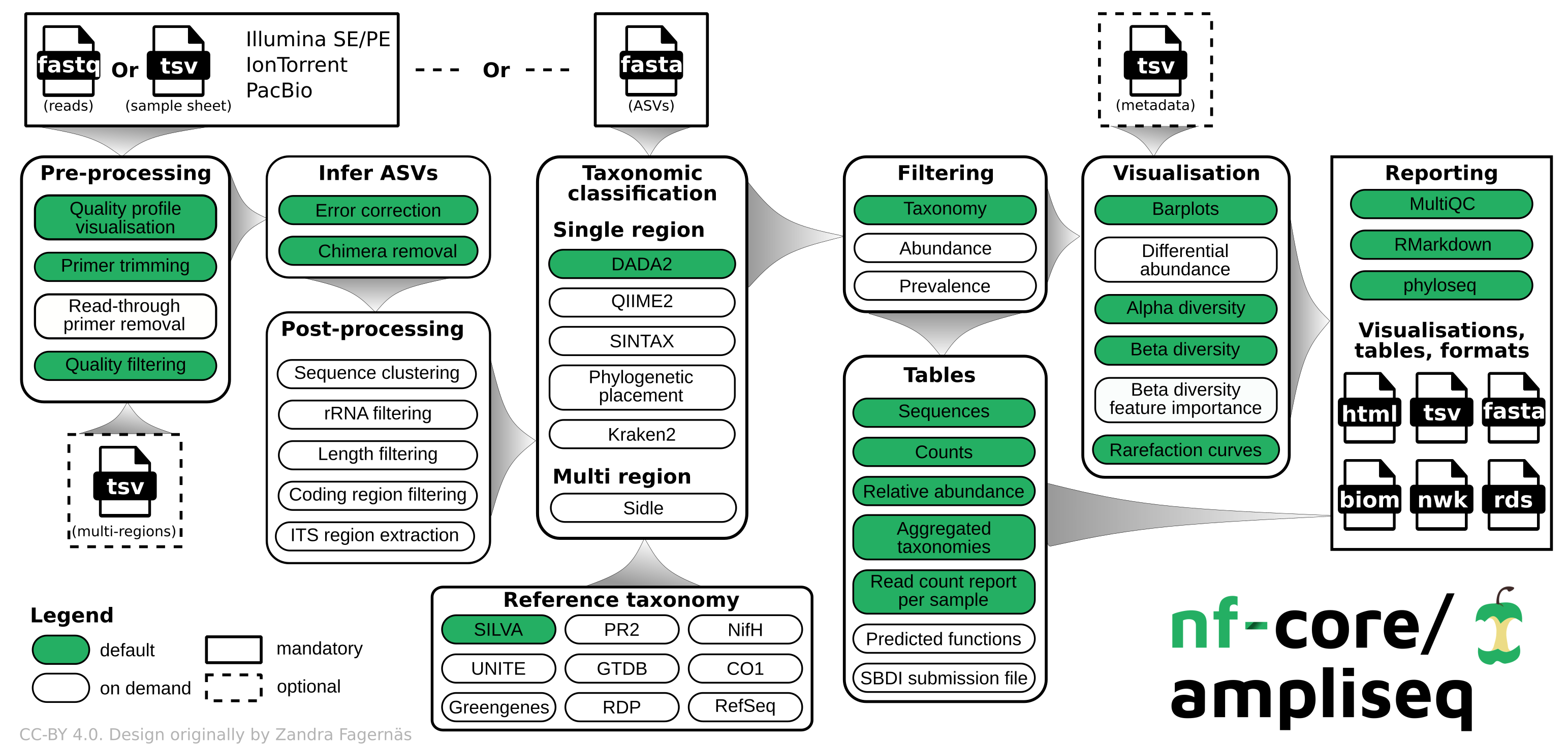
We use ampliseq for the following programs:

• Cutadapt is trimming primer sequences from sequencing reads. Primer sequences are non-biological sequences that often introduce point mutations that do not reflect sample sequences. This is especially true for degenerated PCR primer. If primer trimming would be omitted, artifactual amplicon sequence variants might be computed by the denoising tool or sequences might be lost due to become labelled as PCR chimera.
• DADA2 performs fast and accurate sample inference from amplicon data with single-nucleotide resolution. It infers exact amplicon sequence variants (ASVs) from amplicon data with fewer false positives than many other methods while maintaining high sensitivity. This program also assigns taxonomy using a RDP classifier.

18S primer sequences (required)

Below is what we used for 18S amplicon sequencing. Ampliseq will automatically calculate the reverse compliment and include this for us. Copy the capitalized primer region to place inside the ampliseq script.

Format: lower_case_adapter UPPER_CASE_PRIMER_SEQUENCE

FO4+R22 (Blaxter et al. 1998/Fonseca et al. 2010)
- 18S-SSU-FO4_Illumina (54 bases): tcgtcggcagcgtcagatgtgtataagagacag GCTTGTCTCAAAGATTAAGCC
- 18S-SSU-R22_Illumina (53 bases): gtctcgtgggctcggagatgtgtataagagacag GCCTGCTGCCTTCCTTGGA

v8v9 (Bradley et al. 2016)
- 18S_1422F_illumina (54 bases): tcgtcggcagcgtcagatgtgtataagagacag ATAACAGGTCTGTGATGCCCT
- 18S_1797R_illumina (53 bases): gtctcgtgggctcggagatgtgtataagagacag CTTCYGCAGGTTCACCTAC

Metadata sheet (optional)

The metadata file has to follow the QIIME2 specifications. Below is a preview of the sample sheet used for this test. Keep the column headers the same for future use. The first column needs to be "ID" and can only contain numbers, letters, or "-". This is different than the sample sheet. NAs should be empty cells rather than "NA".

Create samplesheet sheet for ampliseq

This file indicates the sample ID and the path to R1 and R2 files. Below is a preview of the sample sheet used in this test. File created on RStudio Interactive on Discovery Cluster using (create_metadatasheets.R).

• sampleID (required): Unique sample IDs, must start with a letter, and can only contain letters, numbers or underscores (no hyphons!).
• forwardReads (required): Paths to (forward) reads zipped FastQ files
• reverseReads (optional): Paths to reverse reads zipped FastQ files, required if the data is paired-end
• run (optional): If the data was produced by multiple sequencing runs, any string

sampleID	forwardReads	reverseReads	run
sample1	./data/S1_R1_001.fastq.gz	./data/S1_R2_001.fastq.gz	A
sample2	./data/S2_fw.fastq.gz	./data/S2_rv.fastq.gz	A
sample3	./S4x.fastq.gz	./S4y.fastq.gz	B
sample4	./a.fastq.gz	./b.fastq.gz	B

This is an R script, not slurm script. Open RStudio interactive on Discovery Cluster to run this script.

Prior to running R script, use the rawdata file created for the fastqc slurm array from within the raw data folder to create a list of files. Below is an example from our Offshore Wind project but the specifics of the sampleID will be project dependent. This project had four sequencing runs with different file names.

On OOD, open RStudio. Create a new R script file:

03-metadata.R

## Creating ampliseq metadata sheet for GOBLER
## Load libraries 
library(dplyr)
library(stringr)
library(strex) 

### Read in sample sheet 
sample_list <- read.delim2("/projects/gmgi/example/16S/raw_data/rawdata", header=F) %>% 
  dplyr::rename(forwardReads = V1) %>%
  mutate(sampleID = str_after_nth(forwardReads, "data/", 1),

         ### Confirm that _S is correct for your file names, sometimes this is _R
         sampleID = str_before_nth(sampleID, "_S", 1))

         ## add any other mutate functions as needed for sample names
         ## sampleID needs to match a column in your metadata file for later analyses 

# creating sample ID 
sample_list$sampleID <- gsub("-", "_", sample_list$sampleID)

# keeping only rows with R1
sample_list <- filter(sample_list, grepl("R1", forwardReads, ignore.case = TRUE))

# duplicating column 
sample_list$reverseReads <- sample_list$forwardReads

# replacing R1 with R2 in only one column 
sample_list$reverseReads <- gsub("R1", "R2", sample_list$reverseReads)

# rearranging columns 
sample_list <- sample_list[,c(2,1,3)]

sample_list %>% write.csv("/projects/gmgi/example/16S/metadata/samplesheet.csv", 
                          row.names=FALSE, quote = FALSE)

Run nf-core/ampliseq (Cutadapt & DADA2)

Update ampliseq workflow if needed: nextflow pull nf-core/ampliseq.

Create slurm script: nano 04-ampliseq.sh. Copy below script into file and save (Ctrl+X; Y; Enter). You'll notice that /projects/gmgi/Fisheries/scripts/ ampliseq_minBoot.config is used as a custom config file. This file will set minBoot=80 instead of 50 to reflect a more conservative taxonomic assignment.

Set trunclenf and trunclenr based on data quality. Set job name as desired, I use the format ampliseq_<project>_<marker>. Our in-house MiSeq i100 data has been extremely high quality and 250 could be used for trimming.

Either pr2 or pr2=<v#> can be used in the ref taxonomy flag. Ensure the most recent version of pr2 is being used.

skip_summary_report_fastqc is being used right now because this version of ampliseq has a bug in the summary report creation step.

04-ampliseq_16S.sh:

#!/bin/bash
#SBATCH --error=output/"%x_error.%j" #if your job fails, the error report will be put in this file
#SBATCH --output=output/"%x_output.%j" #once your job is completed, any final job report comments will be put in this file
#SBATCH --partition=short
#SBATCH --nodes=1
#SBATCH --time=48:00:00
#SBATCH --job-name=ampliseq_project_marker
#SBATCH --mem=70GB
#SBATCH --ntasks=12
#SBATCH --cpus-per-task=2

### USER TO-DO ### 
## 1. Set paths for project 
## 2. Adjust SBATCH options above (time, mem, ntasks, etc.) as desired  
## 3. Fill in F and R primer information based on primer type (no reverse compliment needed)
## 4. Adjust parameters as needed (below is Fisheries team default for 18S)

# Load nextflow conda environment
source /projects/gmgi/miniconda3/bin/activate nextflow_env

# SET PATHS 
metadata="/projects/gmgi/example/18S/metadata" 
output_dir="/projects/gmgi/example/18S/results"
taxlevels="Domain,Supergroup,Division,Subdivision,Class,Order,Family,Genus,Species"

nextflow run nf-core/ampliseq -resume \
   -c /projects/gmgi/Fisheries/scripts/ampliseq_minBoot.config \
   -profile singularity \
   --input ${metadata}/samplesheet.csv \
   --FW_primer "" \
   --RV_primer "" \
   --outdir ${output_dir} \
   --trunclenf 240 \
   --trunclenr 240 \
   --max_ee 2 \
   --sample_inference pseudo \
   --ignore_failed_trimming \
   --ignore_empty_input_files \
   --dada_ref_taxonomy pr2 \
   --dada_assign_taxlevels ${taxlevels} \
   --skip_summary_report_fastqc true

To run:
- sbatch 04-ampliseq.sh

Files generated by ampliseq

Pipeline summary reports:

• summary_report/
• summary_report.html: pipeline summary report as standalone HTML file that can be viewed in your web browser.
• *.svg*: plots that were produced for (and are included in) the report.
• versions.yml: software versions used to produce this report.

Preprocessing:

• FastQC: fastqc/ and *_fastqc.html: FastQC report containing quality metrics for your untrimmed raw fastq files.
• Cutadapt: cutadapt/ and cutadapt_summary.tsv: summary of read numbers that pass cutadapt
• MultiQC: multiqc, multiqc_data/, multiqc_plots/ with multiqc_report.html: a standalone HTML file that can be viewed in your web browser;

ASV inferrence with DADA2:

• dada2/, dada2/args/, data2/log/
• ASV_seqs.fasta: Fasta file with ASV sequences.
• ASV_table.tsv: Counts for each ASV sequence.
• DADA2_stats.tsv: Tracking read numbers through DADA2 processing steps, for each sample.
• DADA2_table.rds: DADA2 ASV table as R object.
• DADA2_table.tsv: DADA2 ASV table.
• dada2/QC/
• *.err.convergence.txt: Convergence values for DADA2's dada command, should reduce over several magnitudes and approaching 0.
• *.err.pdf: Estimated error rates for each possible transition. The black line shows the estimated error rates after convergence of the machine-learning algorithm. The red line shows the error rates expected under the nominal definition of the Q-score. The estimated error rates (black line) should be a good fit to the observed rates (points), and the error rates should drop with increased quality.
• *_qual_stats.pdf: Overall read quality profiles: heat map of the frequency of each quality score at each base position. The mean quality score at each position is shown by the green line, and the quartiles of the quality score distribution by the orange lines. The red line shows the scaled proportion of reads that extend to at least that position.
• *_preprocessed_qual_stats.pdf: Same as above, but after preprocessing.

We add an ASV length filter that will output asv_length_filter/ with:

• ASV_seqs.len.fasta: Fasta file with filtered ASV sequences.
• ASV_table.len.tsv: Counts for each filtered ASV sequence.
• ASV_len_orig.tsv: ASV length distribution before filtering.
• ASV_len_filt.tsv: ASV length distribution after filtering.
• stats.len.tsv: Tracking read numbers through filtering, for each sample.